Texas Instruments (TI) Calculators for Polynomial Problems

You may use any of these TI calculators:
TI-83 Plus
TI-84 Plus series
TI-Nspire CX series
TI-89 Titanium
TI-73 Explorer

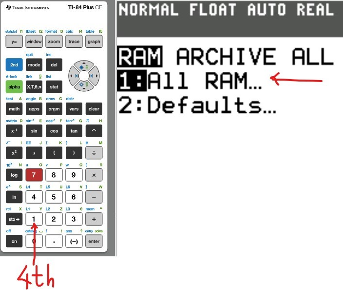
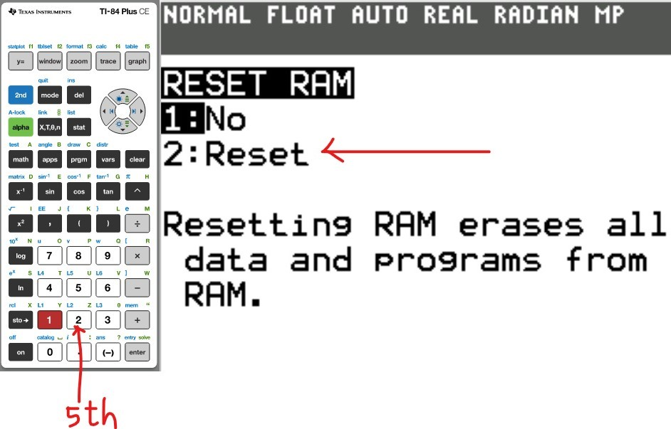
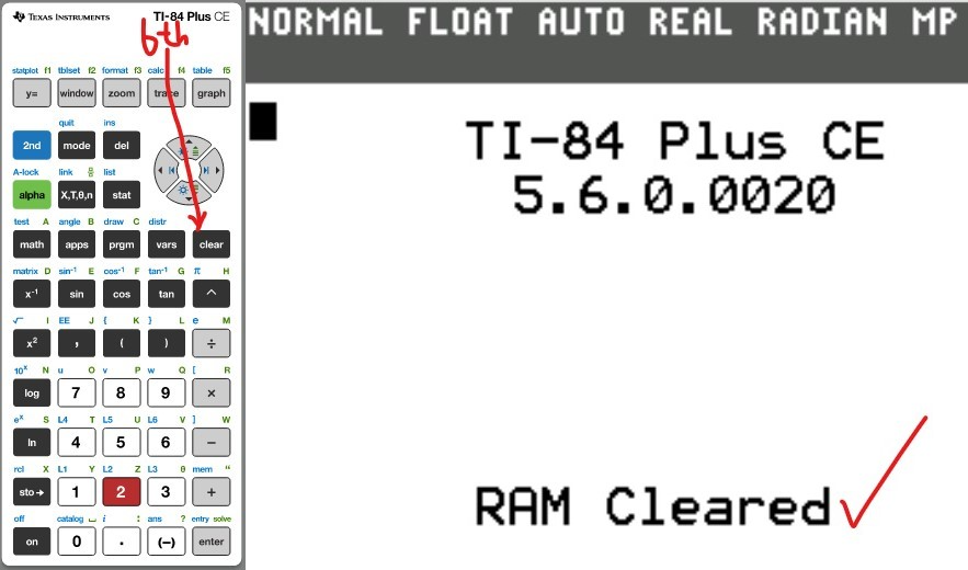
The first thing we need to do is to reset the Random Access Memory (RAM).
This will clear everything that was initially stored by a previous user.
Also, after each problem, it is recommended that you reset the calculator.

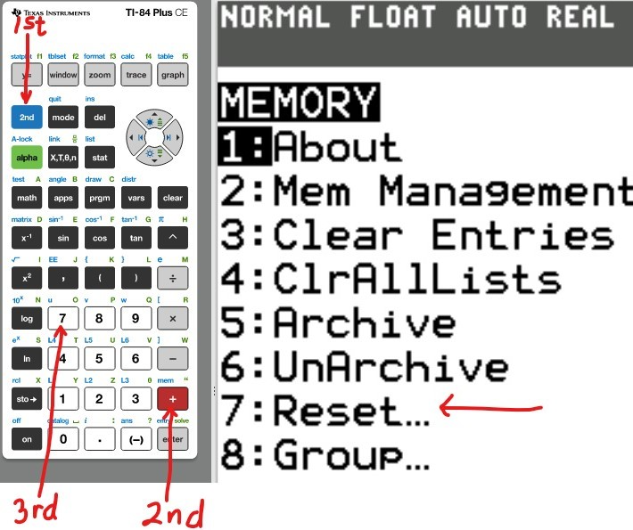
Reset the Calculator
(1.) Reset 1 (2.) Reset 2
(3.) Reset 3 (4.) Reset 4


Let us do some examples.
NOTE: Please begin from the first example. Do not skip.


Concepts: Graph polynomials, Determine local extrema
(a.) Graph a polynomial within a range of values
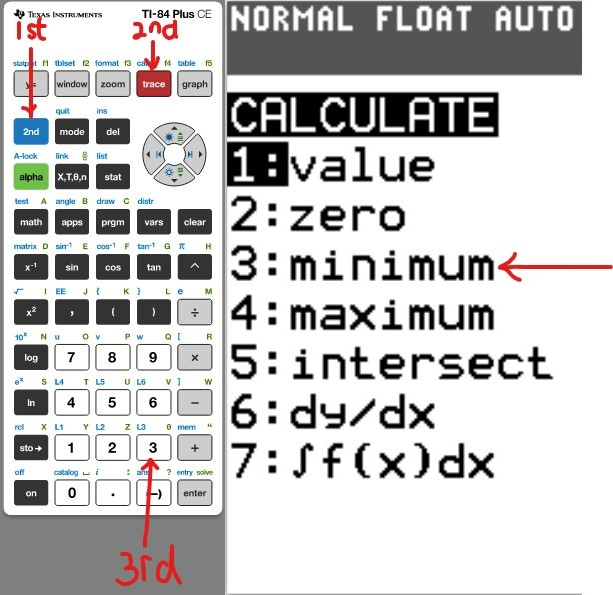
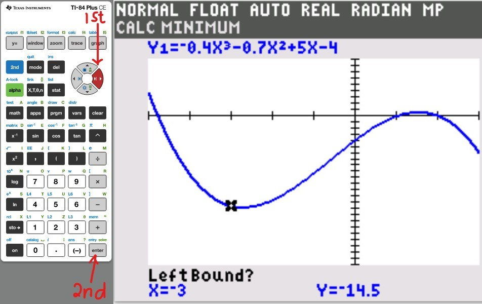
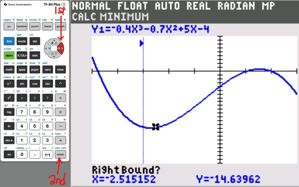
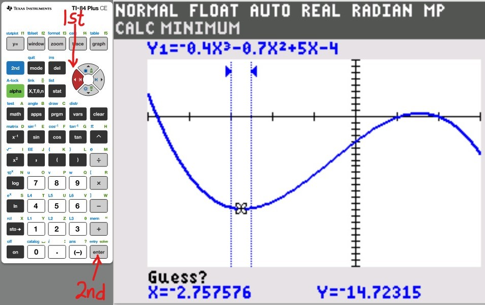
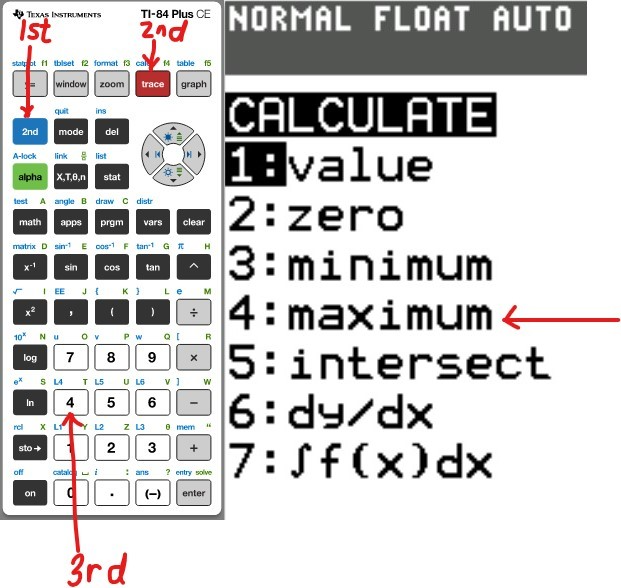
(b.) Determine the local minimum of the polynomial
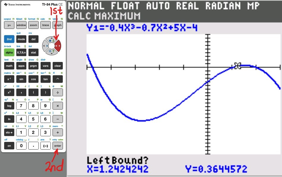
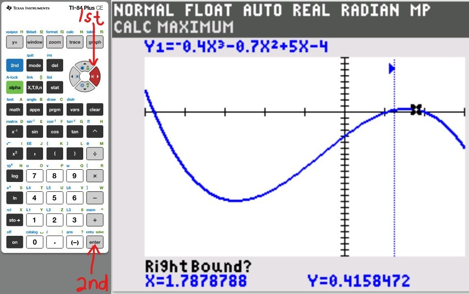
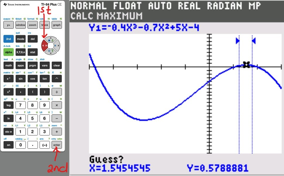
(c.) Determine the local maximum of the polynomial.

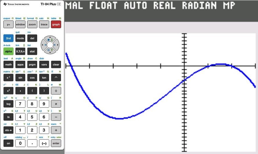
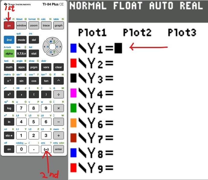
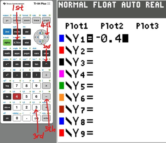
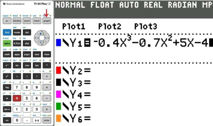
(1.) (a.) Use a graphing utility to approximate the local maximum value and local minimum value of the function $$ f(x) = -0.4x^3 - 0.7x^2 + 5x - 4 \\[3ex] for\;\; -6 \lt x \lt 4 \\[3ex] and\;\; -25 \lt y \lt 10 \\[3ex] $$ Number 1

(b.) The local minimum is y ≈ ............ and it occurs at x ≈ ............

(c.) The local maximum is y ≈ ............ and it occurs at x ≈ ............

(Round to the nearest hundredth as needed)

(a.) Based on the graph from the TI graphing calculator:

Graph 7

The correct option is option B.

(b.)
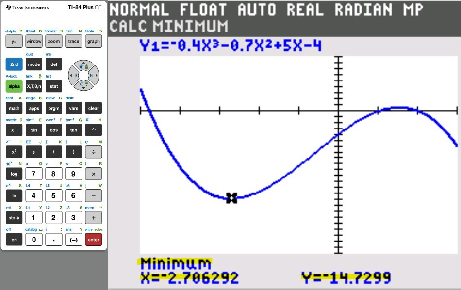
Graph 12

The local minimum is y ≈ −14.73 and it occurs at x ≈ −2.71

(c.)
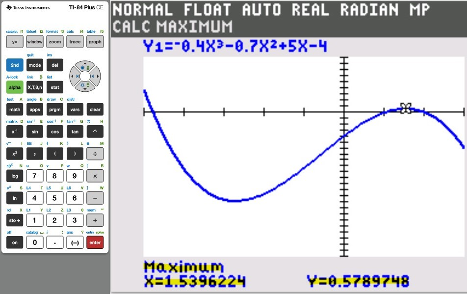
Graph 17

The local maximum is y ≈ 0.58 and it occurs at x ≈ 1.54


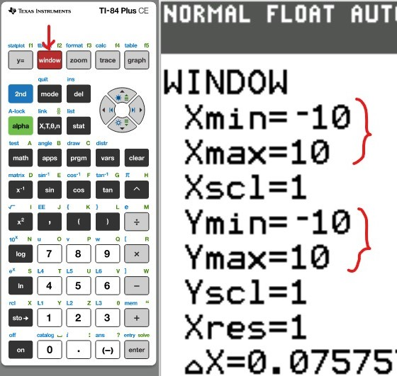
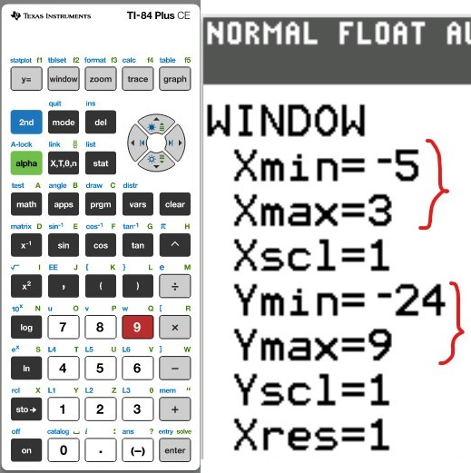
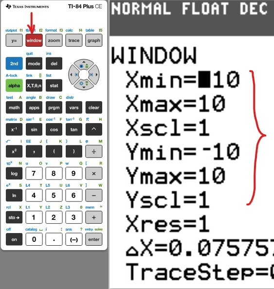
(1.) Graph 1 $X_{min}$ is the minimum value of x on the x-axis
$X_{max}$ is the maximum value of x on the x-axis
$X_{scl}$ is the scale (1 cm to how many units) on the x-axis
$Y_{min}$ is the minimum value of y on the y-ayis
$Y_{max}$ is the maximum value of y on the y-ayis
$Y_{scl}$ is the scale (1 cm to how many units) on the y-axis
$X_{res}$ is the resolution
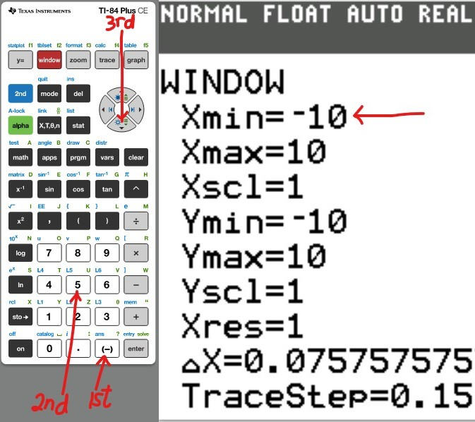
For Question (1.):
−6 < x < 4
$X_{min} = -5$ and $X_{max} = 3$
−25 < y < 10
$Y_{min} = -24$ and $Y_{max} = 9$
(2.) Graph 2 (3.) Graph 3
(4.) Graph 4 (5.) Graph 5
(6.) Graph 6 (7.) Graph 7
(8.) Graph 8 (9.) Graph 9
(10.) Graph 10 (11.) Graph 11
(12.) Graph 12 (13.) Graph 13
(14.) Graph 14 (15.) Graph 15
(16.) Graph 16 (17.) Graph 17


Concept: Model quadratic function
(a.) Develop a quadratic model based on a given data

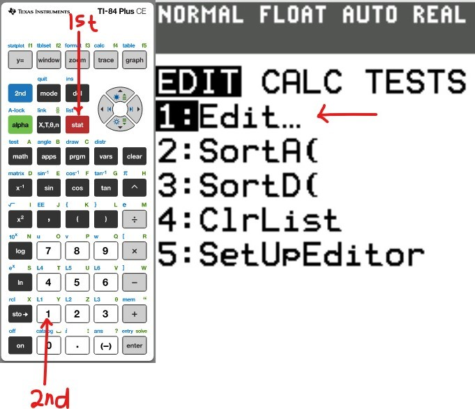
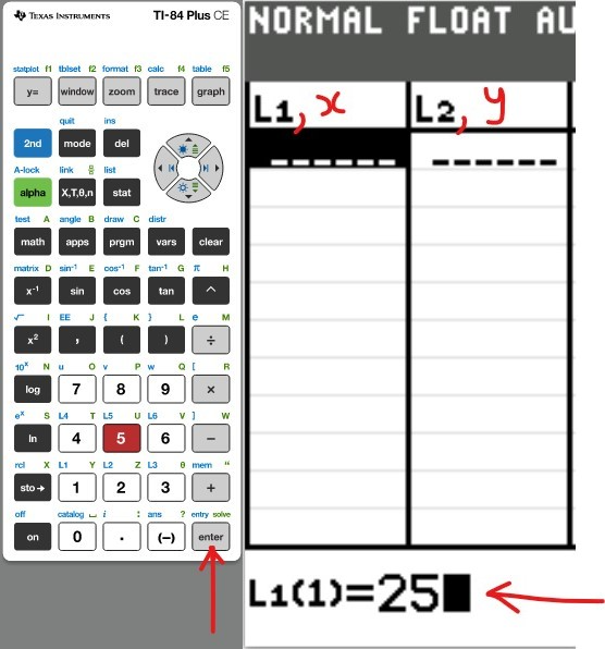
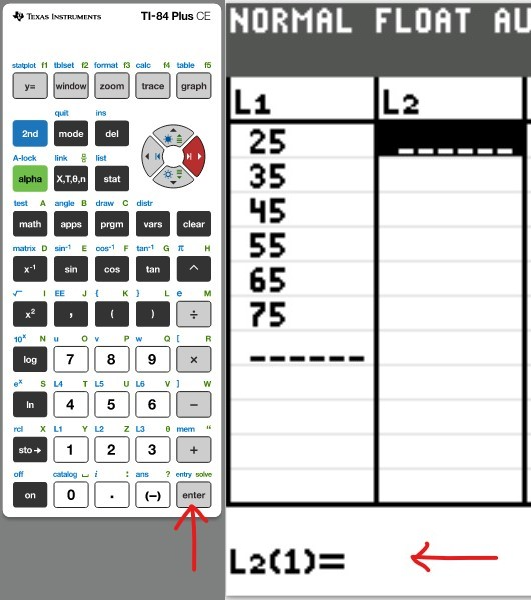
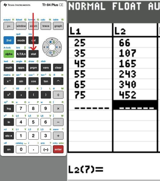
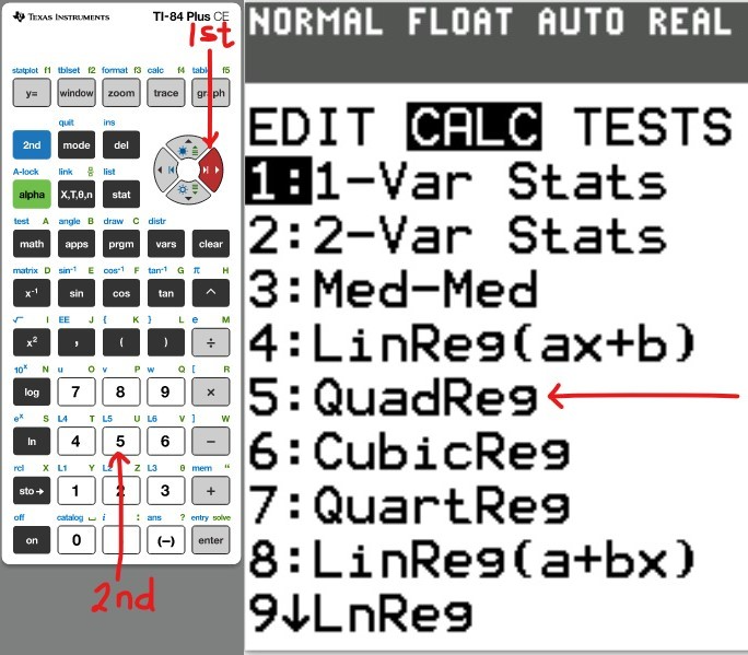
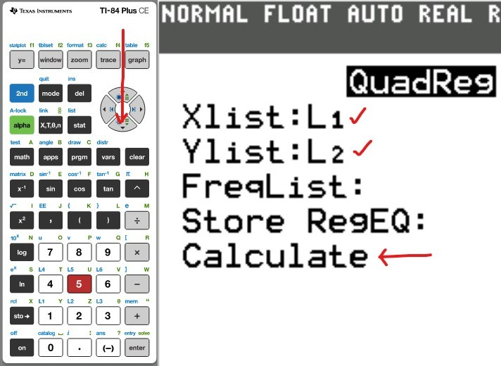
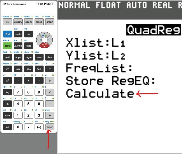
(2.) Use a graphing utility to find the quadratic function of best fit for the data.

x 25 35 45 55 65 75
y 66 107 165 243 340 452


y = .............................
(Type an expression using x as the variable. Use integers or decimals for any numbers in the expression. Round to three decimal places as needed.)

Quadratic Model 8

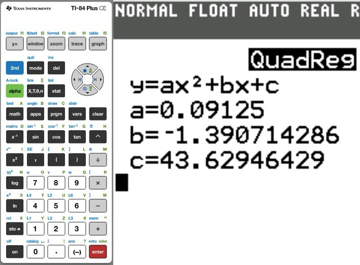
The quadratic function of best fit for the data is:

$ y = ax^2 + bx + c \\[3ex] y = 0.09125x^2 - 1.390714286x + 43.62946429 \\[3ex] y \approx 0.091x^2 - 1.391x +43.629 $


(1.) Quadratic Model 1 (2.) Quadratic Model 2
(3.) Quadratic Model 3 (4.) Quadratic Model 4
(5.) Quadratic Model 5 (6.) Quadratic Model 6
(7.) Quadratic Model 7 (8.) Quadratic Model 8


Concept: Scatter Diagrams
(a.) Draw scatter diagrams
(b.) Interpret scatter diagrams

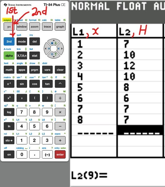
(3.) The following data represent the number of major hurricane strikes in a particular country each decade from 1921 to 2000.

Decade, x Major Hurricanes Striking, H
1921 – 1930, 1 7
1931 – 1940, 2 10
1941 – 1950, 3 12
1951 – 1960, 4 10
1961 – 1970, 5 8
1971 – 1980, 6 6
1981 – 1990, 7 7
1991 – 2000, 8 7


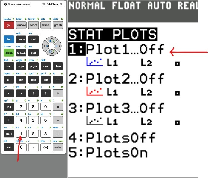
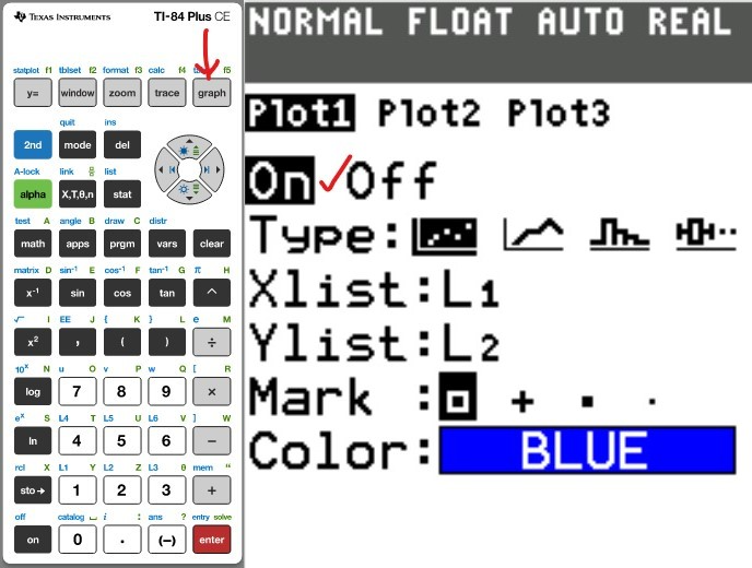
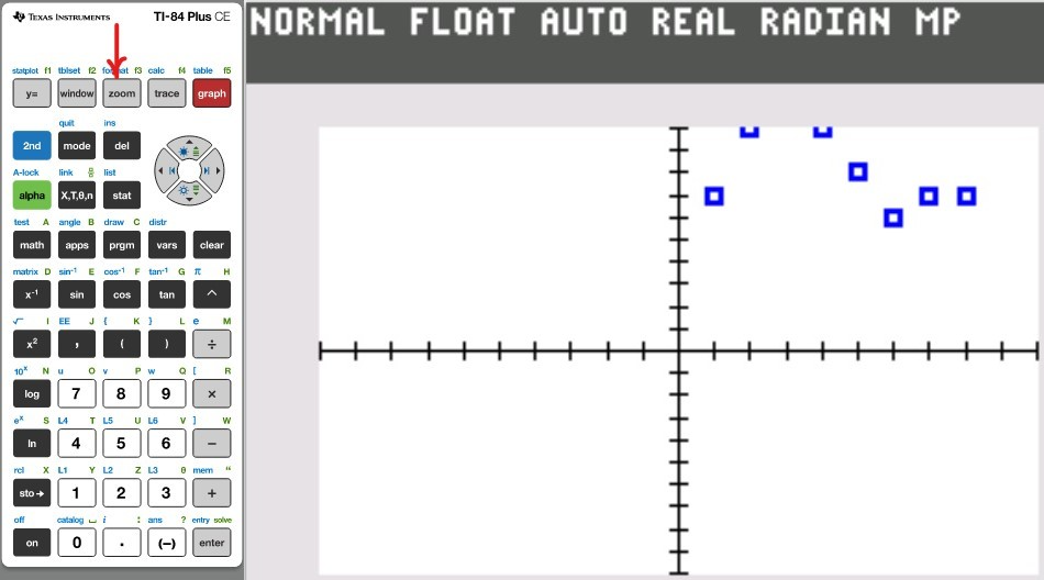
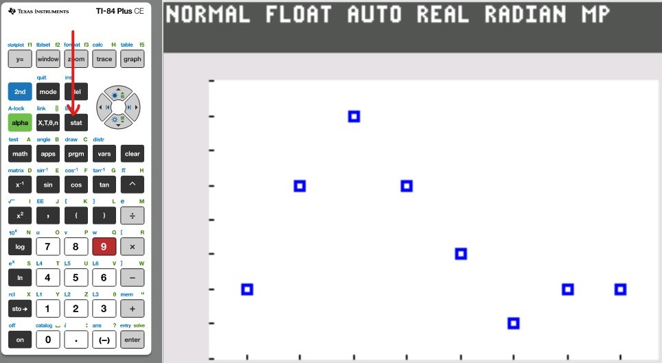
(a.) Draw a scatter diagram of the data.
Comment on the type of relation that may exist between the two variables.
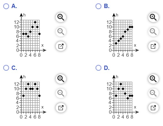
Which of the following shows the correct scatter diagram for these data?

Number 3a

(b.) Which relation best describes these data?
(I.) linear with positive slope
(II.) no relation
(III.) cubic
(IV.) linear with negative slope

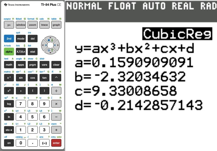
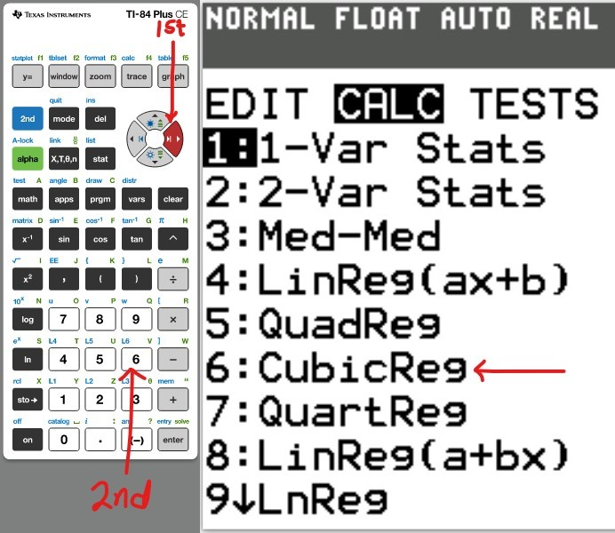
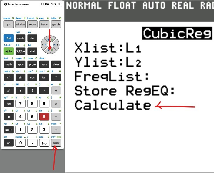
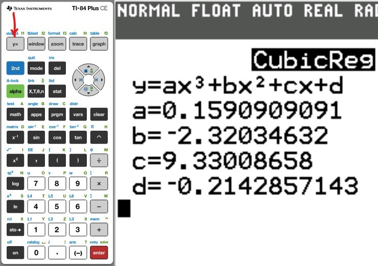
(c.) The cubic function of best fit to these data is

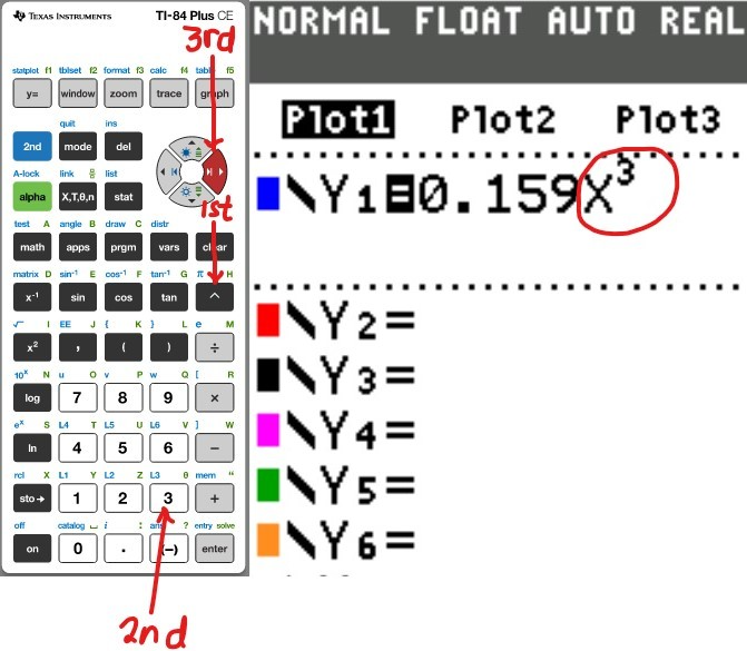
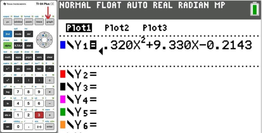
$ H(x) = 0.159x^3 - 2.320x^2 + 9.330x - 0.2143 \\[3ex] $ Use a graphing utility to verify that this is the cubic function of best fit.
Use this function to predict the number of major hurricanes that struck between 1961 – 1970.
............. hurricanes.
(Round to the nearest integer as needed.)

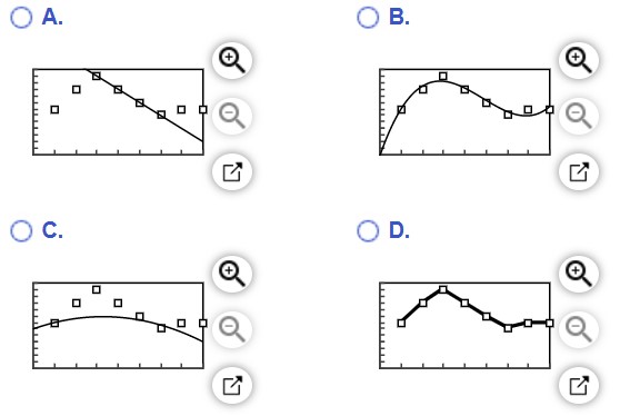
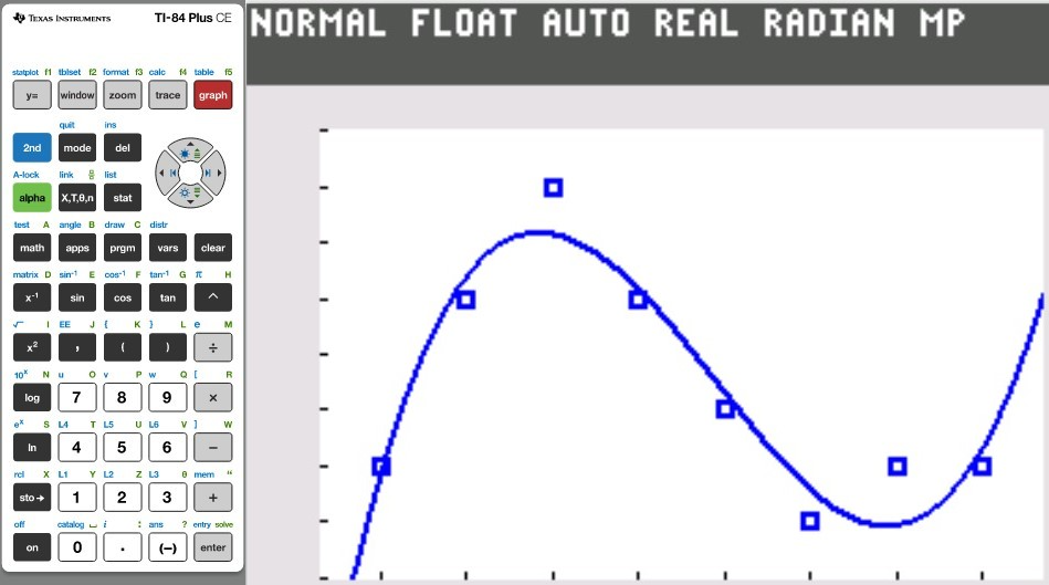
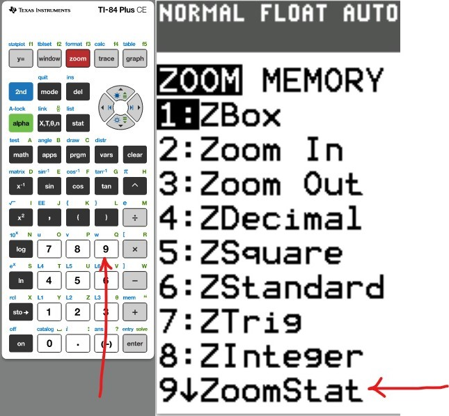
(d.) With a graphing utility, draw a scatter diagram of the data and then graph the cubic function of best fit on the scatter diagram.

Number 3d

(e.) Concern has risen about the increase in the number and intensity of hurricanes, but some scientists believe this is just a natural fluctuation that could last another decade or two.
Use your model to predict the number of major hurricanes that will strike between 2001 and 2010.
(Round to the nearest integer as needed.)

(f.) Does your result appear to agree with what these scientists believe?

(g.) From 2001 – 2005, 6 hurricanes struck.
Does this support or contradict your prediction in part(f)?

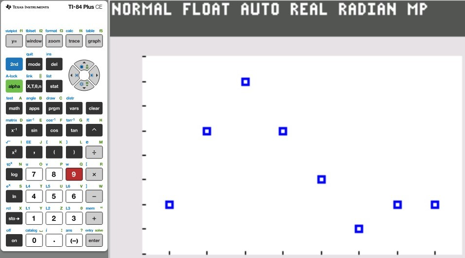
(a.) Based on the scatter diagram from the calculator:
Scatter Diagram 8

The correct option is option D.

(b.) The scatter diagram shows a cubic relationship.

(c.) The cubic function of best fit to these data is

$ H(x) = 0.159x^3 - 2.320x^2 + 9.330x - 0.2143 \\[3ex] $ Use a graphing utility to verify that this is the cubic function of best fit.

Scatter Diagram 12

Use this function to predict the number of major hurricanes that struck between 1961 – 1970.
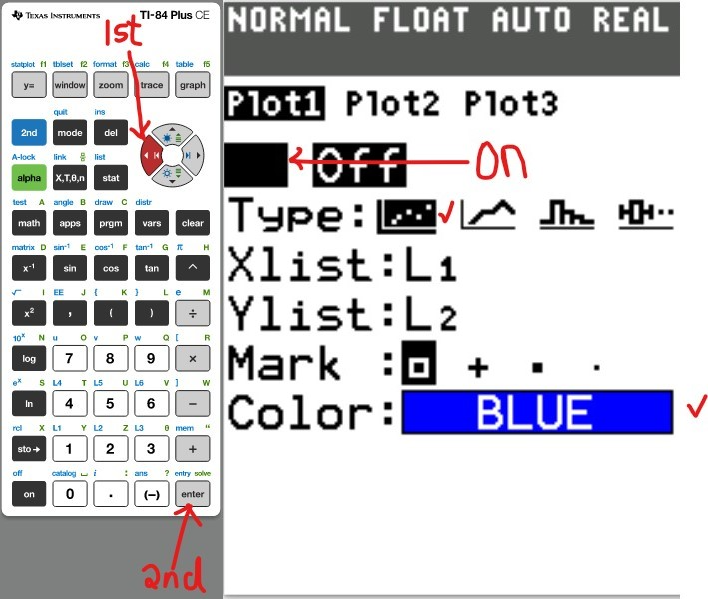
1961 – 1970 ⇒ x = 5

$ H(x) = 0.159x^3 - 2.320x^2 + 9.330x - 0.2143 \\[3ex] H(5) = 0.159(5)^3 - 2.32(5)^2 + 9.33(5) - 0.2143 \\[3ex] = 0.159(125) - 2.32(25) + 46.65 - 0.2143 \\[3ex] = 19.875 - 58 + 46.65 - 0.2143 \\[3ex] = 8.3107 \\[3ex] \approx 8 \\[3ex] $ The number of major hurricanes that struck between 1961 – 1970 is approximately 8 hurricanes.

(d.) The scatter diagram and the graph of the cubic function is:

Scatter Diagram 16

(e.) Following the trend:
2001 – 2010 ⇒ x = 9

$ H(x) = 0.159x^3 - 2.320x^2 + 9.330x - 0.2143 \\[3ex] H(9) = 0.159(9)^3 - 2.32(9)^2 + 9.33(9) - 0.2143 \\[3ex] = 0.159(729) - 2.32(81) + 46.65 - 0.2143 \\[3ex] = 115.911 - 187.92 + 83.97 - 0.2143 \\[3ex] = 11.7467 \\[3ex] \approx 12 \\[3ex] $ The number of major hurricanes that struck between 2001 – 2010 is approximately 12 hurricanes.

(f.) Does your result appear to agree with what these scientists believe?
Yes, the natural fluctuation is supported because the result is comparable to hurricane data from past decades.
There were 12 major hurricanes between 1941 – 1950

(g.) From 2001 – 2005, 6 hurricanes struck.
Does this support or contradict your prediction in part(f)?
Yes, it supports it.
Half of the hurricanes (6) struck in the first half (first 5 years: 2001 – 2005) of the decade.
It is possible that the other half (6) could occur in the second half (second 5 years: 2005 – 2010) of the decade.


(1.) Scatter Diagram 1 (2.) Scatter Diagram 2
(3.) Scatter Diagram 3 (4.) Scatter Diagram 4
(5.) Scatter Diagram 5 (6.) Scatter Diagram 6
(7.) Scatter Diagram 7 (8.) Scatter Diagram 8


The cubic function of best fit to these data is

$ H(x) = 0.159x^3 - 2.320x^2 + 9.330x - 0.2143 \\[3ex] $ Use a graphing utility to verify that this is the cubic function of best fit.

(9.) Scatter Diagram 9 (10.) Scatter Diagram 10
(11.) Scatter Diagram 11 (12.) Scatter Diagram 12


$ y = ax^3 + bx^2 + cx + d \\[3ex] H(x) = 0.1590909091x^3 - 2.32034632x^2 + 9.33008658x - 0.2142857143 \\[3ex] H(x) \approx 0.159x^3 - 2.320x^2 + 9.330x - 0.2143 \\[3ex] $ With a graphing utility, draw a scatter diagram of the data and then graph the cubic function of best fit on the scatter diagram.

(13.) Scatter Diagram 13 (14.) Scatter Diagram 14
(15.) Scatter Diagram 15 (16.) Scatter Diagram 16


Concept: Table of Values
(a.) Given:
(i.) a polynomial
(ii.) several values of x within constant increments

(b.) To Do:
(i) Determine values of y
(ii) Make a Table of Values for the polynomial

(4.) In Calculus, certain functions can be approximated by polynomial functions.
Explore such function now.
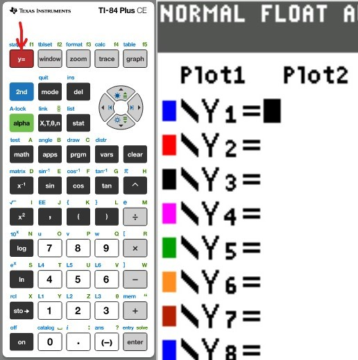
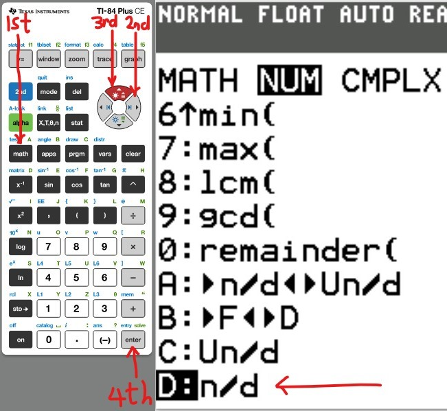
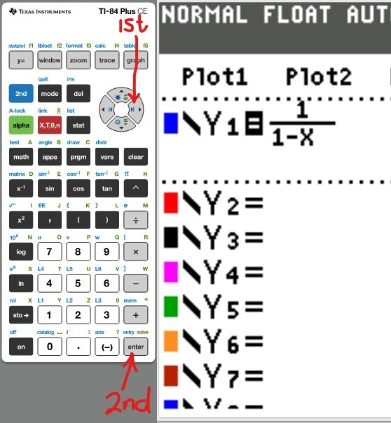
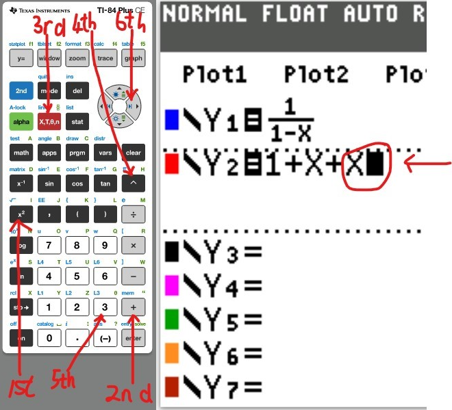
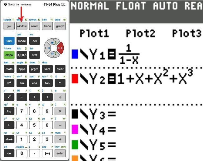
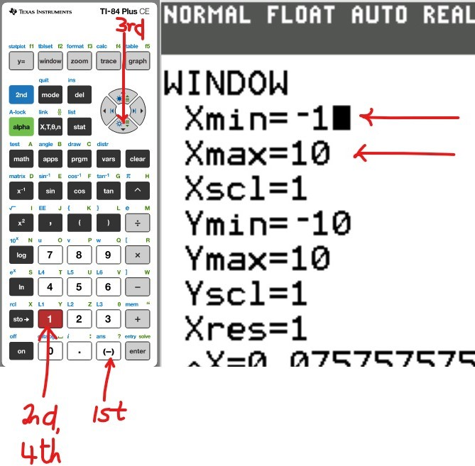
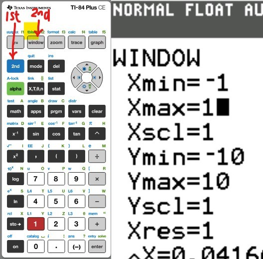
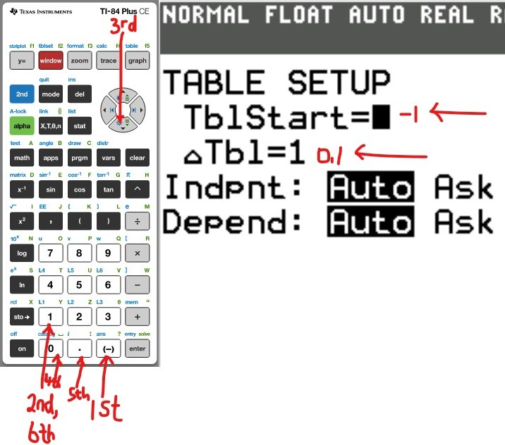
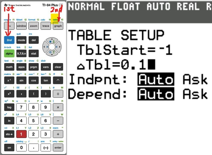
(a.) Using a graphing utility, create a table of values with $Y_1 = f_1(x) = \dfrac{1}{1 - x}$ and $Y_2 = g_1(x) = 1 + x + x^2 + x^3$ for $-1 \le x \le 1$ with $\Delta Tbl = 0.1$
(Type an integer or decimal rounded to five decimal places as needed. Type N if the function is undefined).

$x$ $Y_1$ $Y_2$
−1 ............ ............
−0.9 ............ ............
−0.8 ............ ............
−0.7 ............ ............
−0.6 ............ ............
−0.5 ............ ............
−0.4 ............ ............
−0.3 ............ ............
−0.2 ............ ............
−0.1 ............ ............
0 ............ ............
0.1 ............ ............
0.2 ............ ............
0.3 ............ ............
0.4 ............ ............
0.5 ............ ............
0.6 ............ ............
0.7 ............ ............
0.8 ............ ............
0.9 ............ ............
1 ............ ............


(b.) Using a graphing utility, create a table of values with $Y_1 = f_2(x) = \dfrac{1}{1 - x}$ and $Y_2 = g_2(x) = 1 + x + x^2 + x^3 + x^4$ for $-1 \le x \le 1$ with $\Delta Tbl = 0.1$
(Type an integer or decimal rounded to five decimal places as needed. Type N if the function is undefined).

$x$ $Y_1$ $Y_2$
−1 ............ ............
−0.9 ............ ............
−0.8 ............ ............
−0.7 ............ ............
−0.6 ............ ............
−0.5 ............ ............
−0.4 ............ ............
−0.3 ............ ............
−0.2 ............ ............
−0.1 ............ ............
0 ............ ............
0.1 ............ ............
0.2 ............ ............
0.3 ............ ............
0.4 ............ ............
0.5 ............ ............
0.6 ............ ............
0.7 ............ ............
0.8 ............ ............
0.9 ............ ............
1 ............ ............


(c.) Using a graphing utility, create a table of values with $Y_1 = f_3(x) = \dfrac{1}{1 - x}$ and $Y_2 = g_3(x) = 1 + x + x^2 + x^3 + x^4 + x^5$ for $-1 \le x \le 1$ with $\Delta Tbl = 0.1$
(Type an integer or decimal rounded to five decimal places as needed. Type N if the function is undefined).

$x$ $Y_1$ $Y_2$
−1 ............ ............
−0.9 ............ ............
−0.8 ............ ............
−0.7 ............ ............
−0.6 ............ ............
−0.5 ............ ............
−0.4 ............ ............
−0.3 ............ ............
−0.2 ............ ............
−0.1 ............ ............
0 ............ ............
0.1 ............ ............
0.2 ............ ............
0.3 ............ ............
0.4 ............ ............
0.5 ............ ............
0.6 ............ ............
0.7 ............ ............
0.8 ............ ............
0.9 ............ ............
1 ............ ............


(d.) What do you notice about the values of the function as more terms are added to the polynomial?
Are there some values of x for which the approximations are better?

A. As more terms are added, the values of the polynomial function get further and further away from the values of f.
The approximations near −1 or 1 are better than those near 0.

B. As more terms are added, the values of the polynomial function get closer to the values of f.
The approximations near 0 are better than those near −1 or 1.

C. As more terms are added, the values of the polynomial function get further and further away from the values of f.
The approximations near 0 are better than those near −1 or 1.

D. As more terms are added, the values of the polynomial function get closer to the values of f.
The approximations near −1 or 1 are better than those near 0.
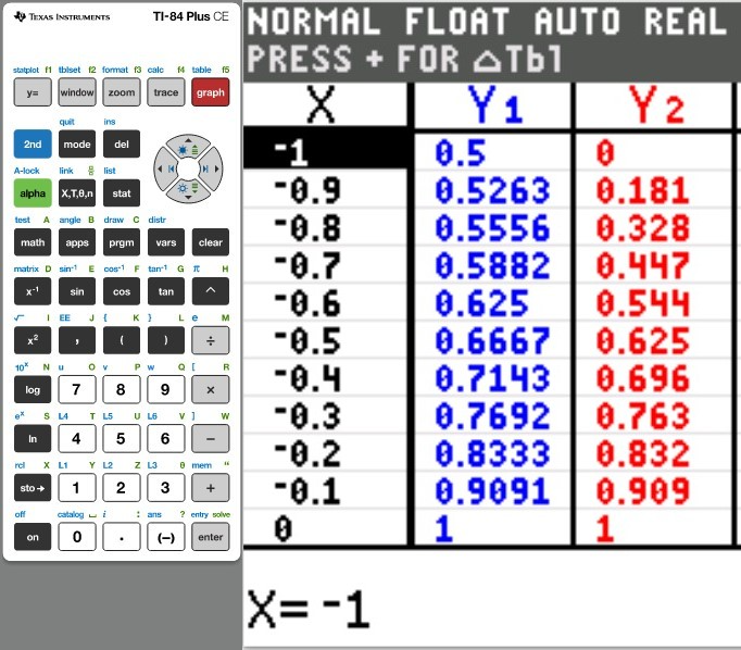
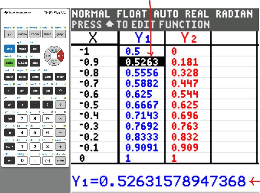
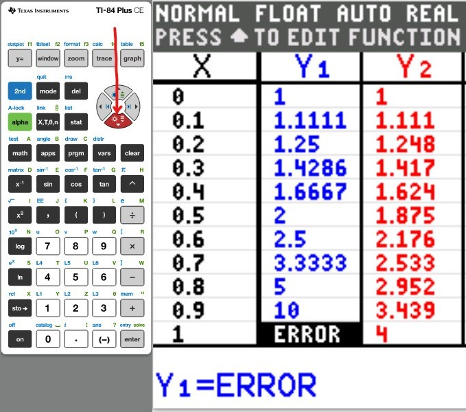
(a.) Table of Values for $Y_1 = f_1(x) = \dfrac{1}{1 - x}$ and $Y_2 = g_1(x) = 1 + x + x^2 + x^3$ for $-1 \le x \le 1$ with $\Delta Tbl = 0.1$

$x$ $Y_1$ $Y_2$
−1 0.5 0
−0.9 0.52632 0.181
−0.8 0.55556 0.328
−0.7 0.58824 0.447
−0.6 0.625 0.544
−0.5 0.66667 0.625
−0.4 0.71429 0.696
−0.3 0.76923 0.763
−0.2 0.83333 0.832
−0.1 0.90909 0.909
0 1 1
0.1 1.11111 1.111
0.2 1.25 1.248
0.3 1.42857 1.417
0.4 1.66667 1.624
0.5 2 1.875
0.6 2.5 2.176
0.7 3.33333 2.533
0.8 5 2.952
0.9 10 3.439
1 N 4


(b.) Table of Values for $Y_1 = f_2(x) = \dfrac{1}{1 - x}$ and $Y_2 = g_2(x) = 1 + x + x^2 + x^3 + x^4$ for $-1 \le x \le 1$ with $\Delta Tbl = 0.1$

$x$ $Y_1$ $Y_2$
−1 0.5 1
−0.9 0.52632 0.8371
−0.8 0.55556 0.7376
−0.7 0.58824 0.6871
−0.6 0.625 0.6736
−0.5 0.66667 0.6875
−0.4 0.71429 0.7216
−0.3 0.76923 0.7711
−0.2 0.83333 0.8336
−0.1 0.90909 0.9091
0 1 1
0.1 1.11111 1.1111
0.2 1.25 1.2496
0.3 1.42857 1.4251
0.4 1.66667 1.6496
0.5 2 1.9375
0.6 2.5 2.3056
0.7 3.33333 2.7731
0.8 5 3.3616
0.9 10 4.0951
1 N 5


(c.) Table of Values for $Y_1 = f_3(x) = \dfrac{1}{1 - x}$ and $Y_2 = g_3(x) = 1 + x + x^2 + x^3 + x^4 + x^5$ for $-1 \le x \le 1$ with $\Delta Tbl = 0.1$

$x$ $Y_1$ $Y_2$
−1 0.5 0
−0.9 0.52632 0.24661
−0.8 0.55556 0.40992
−0.7 0.58824 0.51903
−0.6 0.625 0.59584
−0.5 0.66667 0.65625
−0.4 0.71429 0.71136
−0.3 0.76923 0.76867
−0.2 0.83333 0.83328
−0.1 0.90909 0.90909
0 1 1
0.1 1.11111 1.11111
0.2 1.25 1.24992
0.3 1.42857 1.42753
0.4 1.66667 1.65984
0.5 2 1.96875
0.6 2.5 2.38336
0.7 3.33333 2.94117
0.8 5 3.68928
0.9 10 4.68559
1 N 6


(d.) Based on the observations of the three tables, we notice that:
As more terms are added, the values of the polynomial function get closer to the values of f.
The approximations near 0 are better than those near −1 or 1.


(1.) Table of Values 1 (2.) Table of Values 2
(3.) Table of Values 3 (4.) Table of Values 4
(5.) Table of Values 5 (6.) Table of Values 6
(7.) Table of Values 7 (8.) Table of Values 8
(9.) Table of Values 9 (10.) Table of Values 10
(11.) Table of Values 11 (12.) Table of Values 12


Concepts: Graph Polynomials on the same Graph; Determine the Point of Intersection
(a.) Graph two polynomial functions
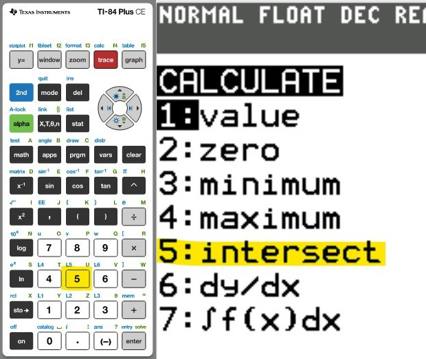
(b.) Determine the point of intersection of the two graphs using the INTERSECT feature

(5.) A golf ball is hit with an initial velocity of 130 feet per second at an inclination of 45° to the horizontal.
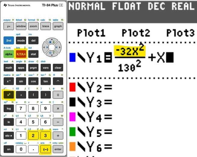
In Physics, it is established that the height of the golf ball is given by the function $$ h(x) = \dfrac{-32x^2}{130^2} + x, $$ where x is the horizontal distance that the golf ball has travelled.

(a.) Determine the height of the golf ball after it has traveled 100 feet.
(Round to two decimal places as needed.)

(b.) What is the height after it has traveled 250 feet?
(Round to two decimal places as needed.)

(c.) What is h(350)?
Interpret this value.
(Round to two decimal places as needed.)

(d.) How far was the golf ball hit?

(Round to two decimal places as needed.)

(e.) Use a graphing utility to graph the function h = h(x)
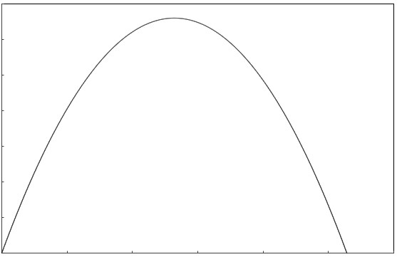
Choose the correct graph below.
[0, 600] by [0, 140], Xscl = 100, Yscl = 20

(f.) Use a graphing utility to determine the distance that the ball has traveled when the height of the ball is 80 feet.
(Round to two decimal places as needed.)

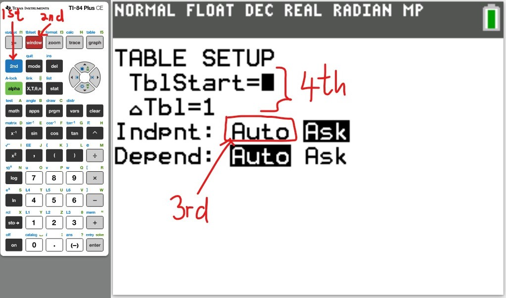
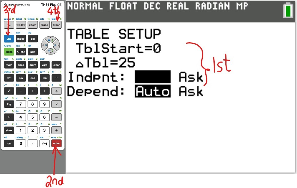
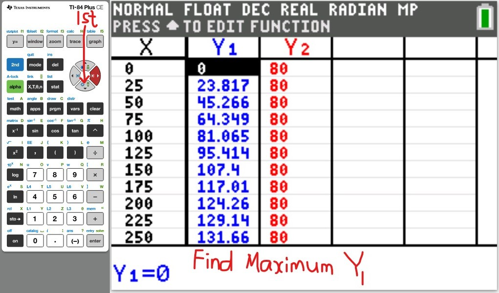
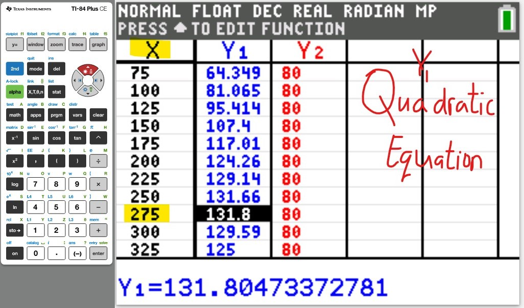
(g.) Create a TABLE with TblStart = 0 and ▵Tbl = 25
(I.) To the nearest 25 feet, how far does the ball travel before it reaches a maximum height?
(II.) To two decimal places as needed, what is the maximum height?

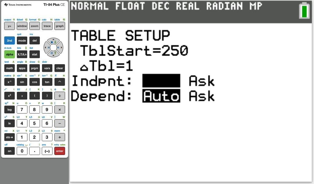
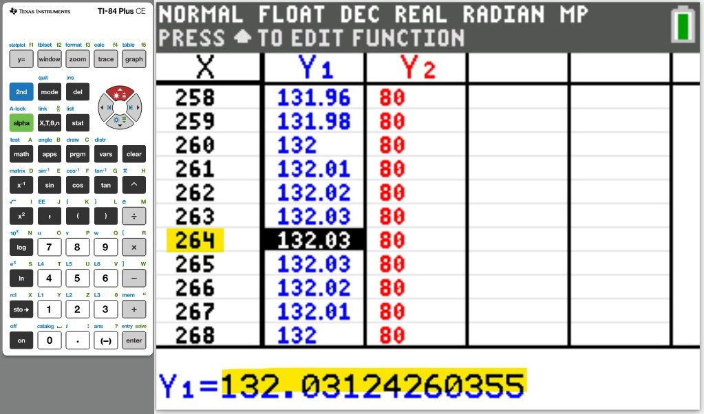
(h.) Adjust the value of ▵Tbl until you determine the​ distance, to within 1​ foot, that the ball travels before it reaches a maximum height.
(I.) To the nearest feet, how far does the ball travel before it reaches a maximum height?
(II.) To two decimal places as needed, what is the maximum height?

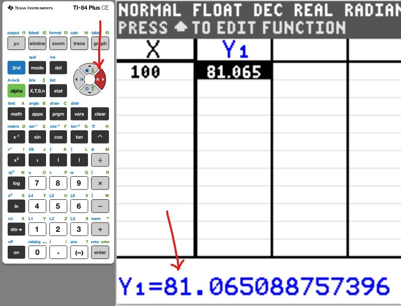
(a.)
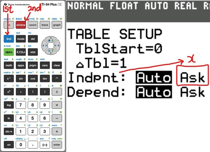
Ask 11
h = 81.065088757396
h ≈ 81.07 feet

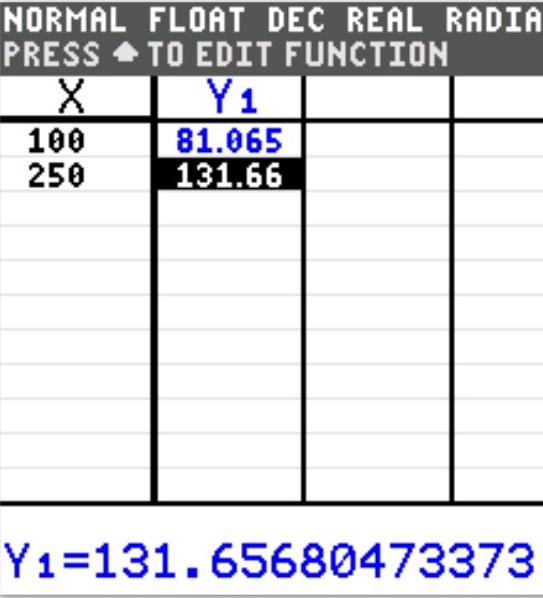
(b.)
Ask 12
h = 131.65680473372
h ≈ 131.66 feet

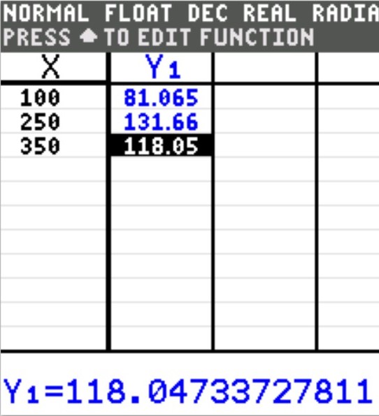
(c.)
Ask 13
h = 118.04733727811
h ≈ 118.05 feet
Interpretation: The height of the golf ball after it has traveled a horizontal distance of 350 feet is approximately 118.05 feet.

(d.)
How far = Distance
How long = Time
How fast = Speed

When the golf ball lands on the ground, the height is 0 feet.
Let us set the height to zero so we can find the distance traveled by the golf ball.

$ h(x) = \dfrac{-32x^2}{130^2} + x \\[5ex] h = 0 \\[3ex] \dfrac{-32x^2}{130^2} + x = 0 \\[5ex] \dfrac{-32x^2}{16900} + x = 0 \\[5ex] \dfrac{-32x^2}{16900} + \dfrac{16900x}{16900} = 0 \\[5ex] \dfrac{-32x^2 + 16900x}{16900} = 0 \\[5ex] -32x^2 + 16900x = 0 \\[3ex] -4x(8x - 4225) = 0 \\[3ex] -4x = 0 \;\;\;OR\;\;\; 8x - 4225 = 0 \\[3ex] x = 0 \;\;\;OR\;\;\; 8x = 4225 \\[3ex] Distance,\;x \;\;cannot\;\;be\;\;0...Discard\;\;0 \\[3ex] 8x = 4225 \\[3ex] x = \dfrac{4225}{8} \\[5ex] x = 528.125 \\[3ex] x \approx 528.13\;feet \\[3ex] $ (e.)
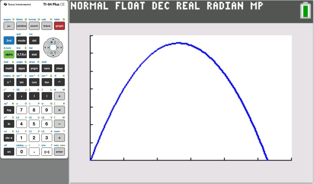
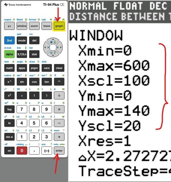
[0, 600] by [0, 140], Xscl = 100, Yscl = 20 means:
Xmin = 0
Xmax = 600
Xscl = 100
Ymin = 0
Ymax = 140
Yscl = 20

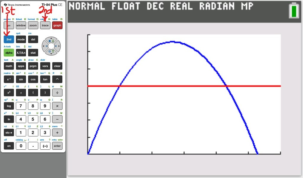
The graph is:
Ask 16

Reviewing all the options, the correct answer is Option B.
Number 5e

(f.)
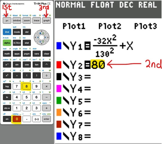
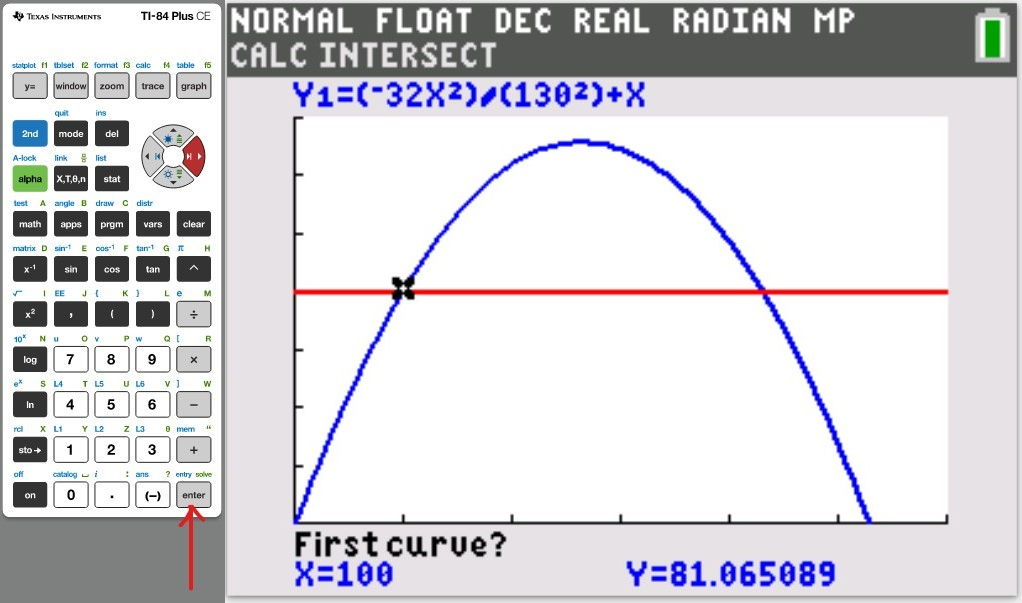
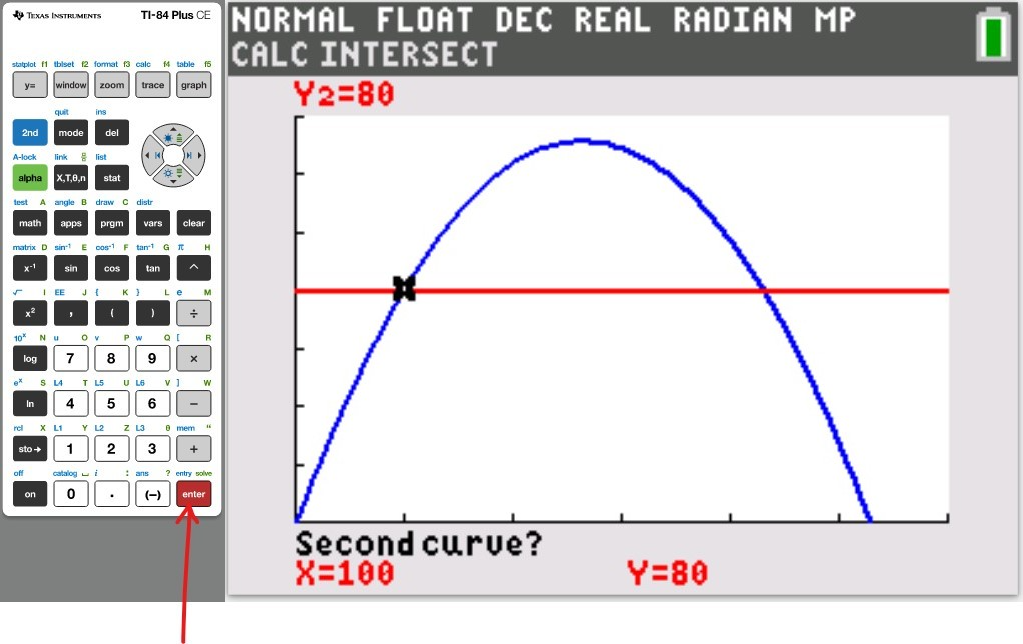
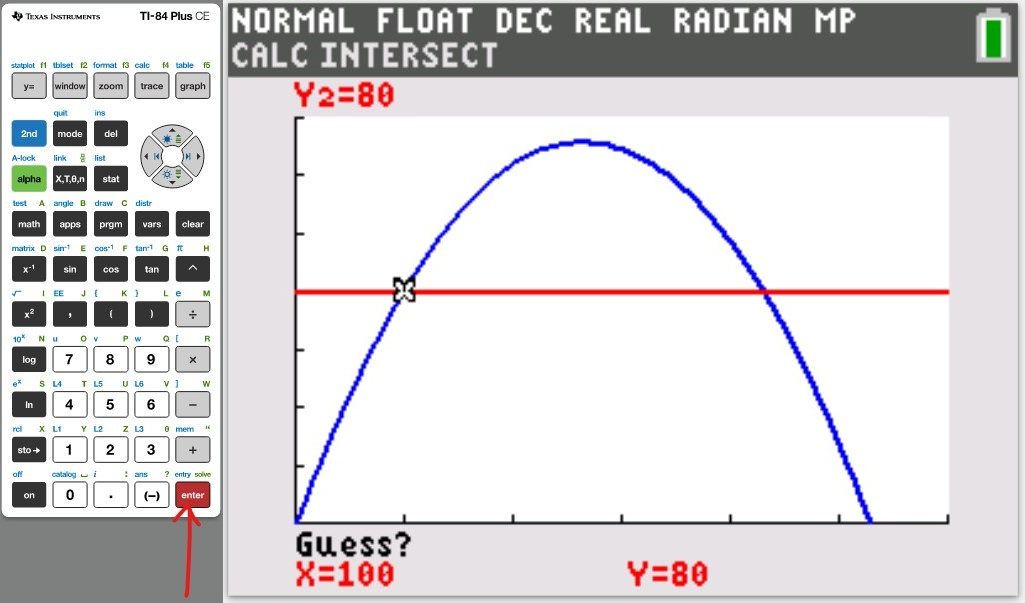
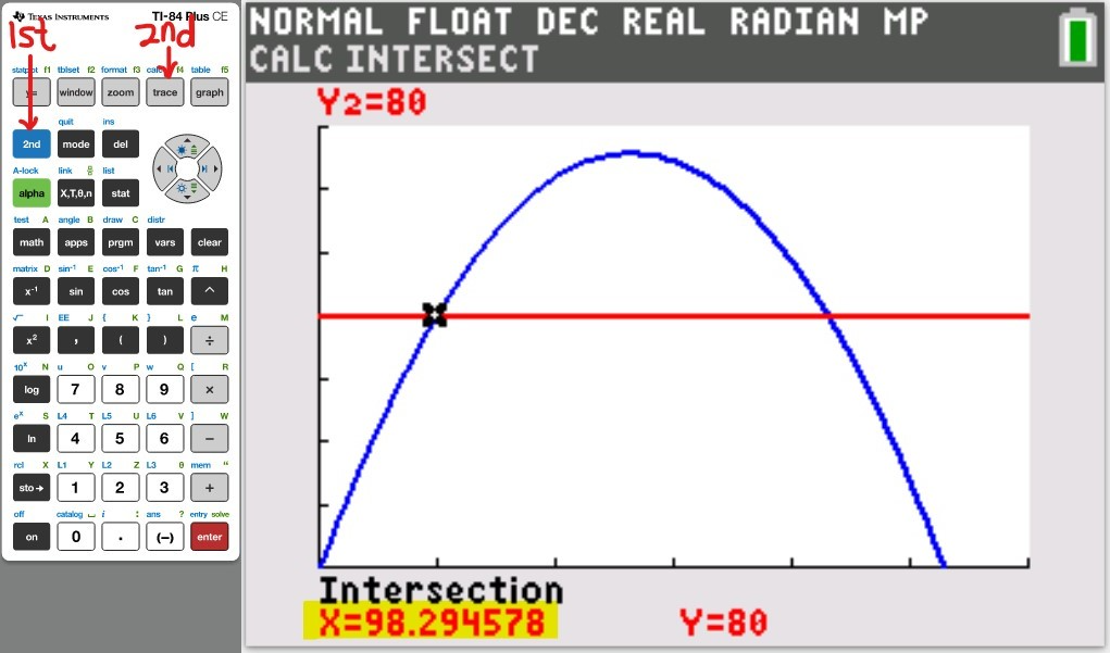
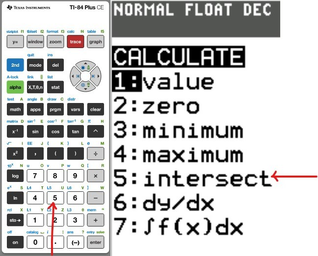
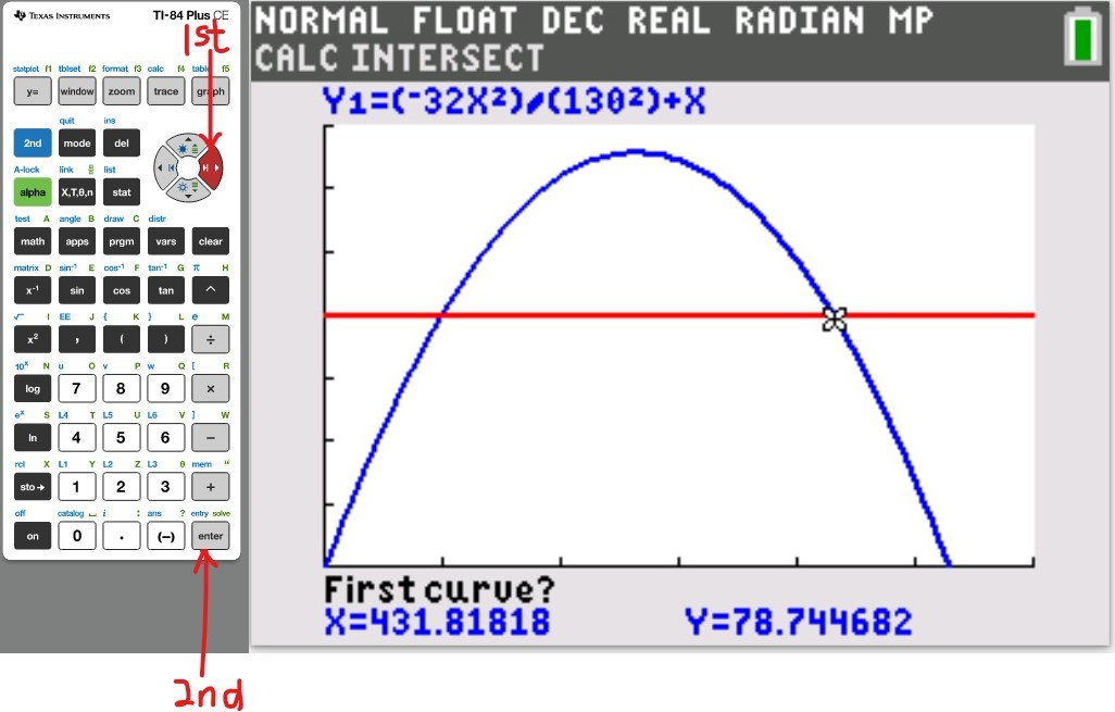
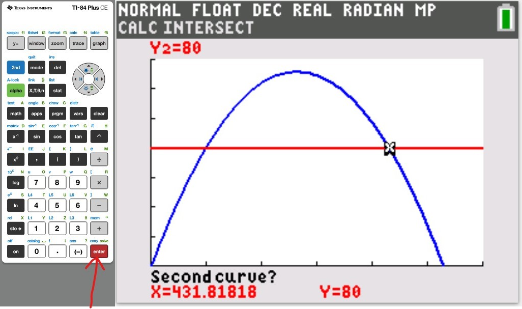
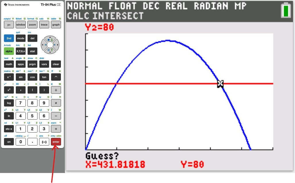
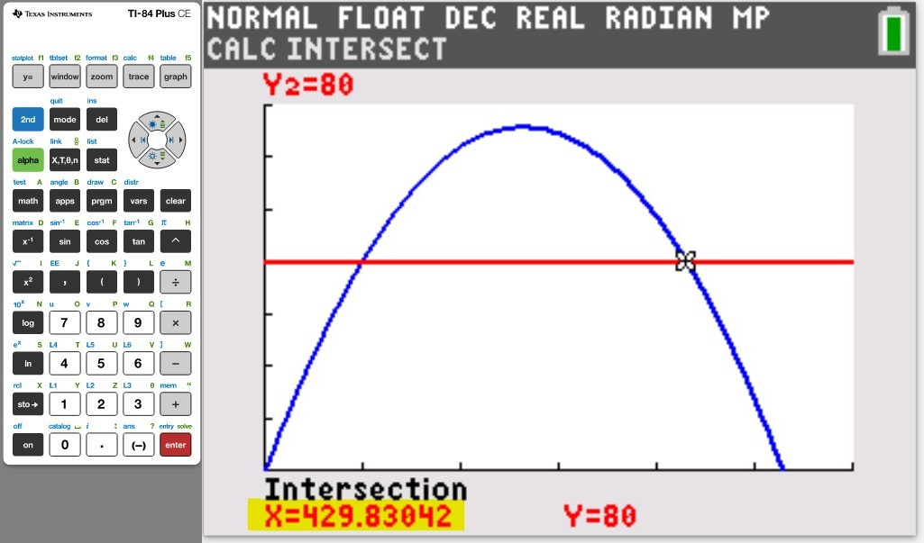
We need to determine the intersection of the two graphs of the functions:

$ h(x) = \dfrac{-32x^2}{130^2} + x \\[5ex] h(x) = 80 \\[3ex] $ (g.) The question wants us to calculate the approximate value of the vertex.
(I.) To the nearest 25 feet, how far does the ball travel before it reaches a maximum height?
To the nearest 25​ feet, the ball travels 275 feet.

(II.) To two decimal places as needed, what is the maximum height? To two decimal places as needed, the maximum height is 131.8 feet

(h.) The question wants us to determine the exact values of the vertex.
Let us set the TblStart to a value close to 275, say 250 and the increment: ▵Tbl = 1
(I.) To the nearest feet, how far does the ball travel before it reaches a maximum height?
To the nearest feet, the ball travels 264 feet.

(II.) To two decimal places as needed, what is the maximum height? To two decimal places as needed, the maximum height is 132.03 feet


Numbers 5(a.) – (c.), (e.)
Let Y = h(x)

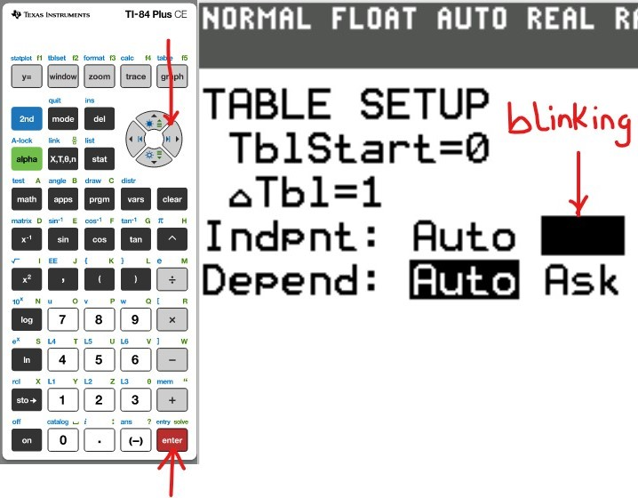
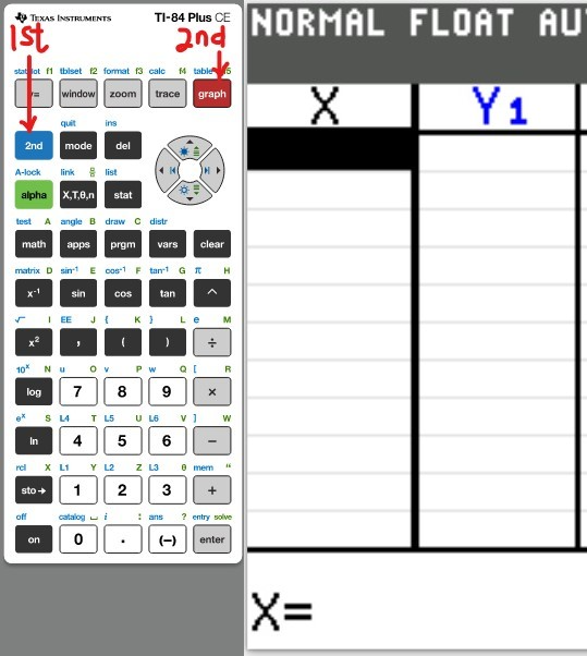
(1.) Ask 1 (2.) Ask 2
(3.) Ask 3 (4.) Ask 4
(5.) Ask 5 (6.) Ask 6
(7.) Ask 7 (8.) Ask 8
(9.) Ask 9 (10.) Ask 10
(11.) Ask 11 (12.) Ask 12
(13.) Ask 13 (14.) Ask 14
(15.) Ask 15 (16.) Ask 16


Number 5(f.)
Intersection of the two graphs:

$ h(x) = \dfrac{-32x^2}{130^2} + x \\[5ex] h(x) = 80 \\[3ex] $
(1.) Intersect 1
(2.) Intersect 2
(3.) Intersect 3
(4.) Intersect 4
(5.) Intersect 5
(6.) Intersect 6
(7.) Intersect 7
(8.) Intersect 8
(9.) Intersect 9
(10.) Intersect 10
(11.) Intersect 11
(12.) Intersect 12
(13.) Intersect 13


Number 5(g.)
First Step to calculate the vertex of the quadratic function:
The vertex is approximate (not exact)

$ h(x) = \dfrac{-32x^2}{130^2} + x \\[5ex] $
(1.) Solve 1
(2.) Solve 2
(3.) Solve 3
(4.) Solve 4


Number 5(h.)
Second Step to calculate the vertex of the quadratic function:
The vertex is exact

$ Let:\;\;TblStart = 250 \\[3ex] \delta Tbl = 1 \\[3ex] h(x) = \dfrac{-32x^2}{130^2} + x \\[5ex] $
(1.) Solve 5
(2.) Solve 6


(6.)


(7.)